This analysis was inspired by a set of talks by Mike Brown of Caltech on small bodies in the Solar System (these are available as part of his course on The Science of the Solar System on Coursera). He speaks with passion about these fascinating objects and how they tell an intriguing story about the formation of our Solar System. Most of the science you’ll meet within this blog comes either from this course or else an excellent book, Physics and Chemistry of the Solar System by John Lewis.
The data come from NASA (where else) and contains information on over 35,000 meteorites up to end 2015. In terms of munging, the data is:
rescaled for meteorite mass in kilogrammes
locations (in longitude/latitude) are attributed to their continents (using a function from Andy South)
some meteors were missing geographical coordinates, an attempt was made to find these and fill them in. This worked for the Nunatak and Yamato fields, both in Antarctica
cleaned to remove remaining incomplete records (6297 of them)
meteorite classes are grouped together. For example, Iron IIIAB, Iron IAB, Iron IC, …. are all just called Irons.
meteorites are further grouped into Chondrite, Achondrites, and Irons (with some subclasses of achondrite based on metal content as there are so many achondrites)
we delete meteorites with a mass of 0kg. There are a handful of these and they mess up our analysis somewhat and are obviously physically impossible
there are a large number (6164) where the (longitude, latitude) is given as (0\(^{\circ}\), 0\(^{\circ}\)). These get dumped in the Atlantic Ocean, just off the coast of Ghana (see the bright red dot in the middle of the map). The name of the meteorite should help locate them, at some point I’ll do something about that. Lots of them are in Antarctica.
Geographical Spread
First, let’s look at where meteorites have been found. The map below shows our meteors. The circle sizes correspond to meteor mass (though you have to zoom in a bit to appreciate the different sizes), the colour indicates the year of discovery. You can click on circles to get these details, as well as the meteor name. To avoid map navigation being tediously slow, only the heaviest meteorites are initially shown, but by clicking the top right legend you can include more.
Map Analysis
The most striking feature of the map is the range in sizes of meteorites, from ones like the giant Hoba weighing in at tens of tonnes to more common, gram-sized meteorites.
Next, we see areas with lots of red, where meteorites have been found more recently: throughout the Sahara, in Antarctica, and across the South central plain of Australia. These are locations in which bizarre looking rocks really stand out in places where they have no right to be. Antarctica has the further advantage that meteorite finds will gather at the foot of glaciers. Surprisingly, there isn’t that much in Greenland, maybe an untapped resource here.
Zooming in on North America, we notice the abundance of kilogramme-sized meteorites discovered in the mid-West throughout the 20th century.
For older meteorite discoveries, we look to Western Europe, the Eastern seaboard of the United States, the Indian subcontinent, and Japan.
In short, meteorites have been found where, a) there are lots of people, or b) they stand out.
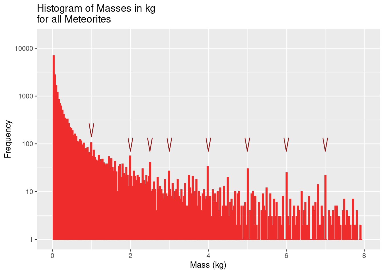
Mass Distribution
Below we show a portion of a histogram of meteorite masses. It shows a predictable ~exponential decline. Note also, anomolously large numbers of meteorites with masses of exactly 1kg, 2kg….(indicated by ticks). My guess is that these were older samples with less rigorous mass measurements.
By Continent
Let’s look at the spread of meteorite mass across different continents. This is shown in the figure below.

Not much to see here. North America is the place to go for larger meteorites, but note the plethora of small meteorites from Antarctica. In fact, by far the greatest number of meteorites come from Antarctica (23368 of them out of a total number of 39018), something that’s hard to appreciate from the map above because they are frequently ascribed the same latitude, longitude and so their pointers sit on top of each other.
Falls versus Finds
There are two categories of meteorites; those that we happen to come across by chance (finds), and those meteors that we see in descent, track, and discover based on their trajectory (falls). Is there a difference in mass? Let’s see.
What we observe is that smaller meteorites tend to be finds. It’s difficult to track meteors, especially in the final, dark, part of their descent when the meteor velocity drops below 3m/s and the visible trail disappears. Unless they are large enough, or unless the terrain is suitable, they won’t be uncovered.
Are We Running Out of Meteorites to Find?
If so we should see a drop off in meteorite mass over time. So let’s plot meteorite mass as a function of year of discovery. It’s shown below (in the plot we also distinguish between different types of meteorite by colour, more on that later):

There appears to be lots of structure in the plot. First off, something dramatic happened from the mid 1970’s on. We begin to see years with enormous numbers of small meteorite discovery. On investigation, these are due to years in which there are meteorite campaigns in Antarctica. Most notable is the Yamato campaign of 1979 that yielded 2935 meteorites with a combined mass of 301.14 kg. Then there was the Asuka campaign of 1988 with 1262 meteorites with a combined mass of 246.18 kg.
We also see some horizontal stripping in this plot. This is due to rounding off measurements of meteorite mass as mentioned above.
The colours in the plot describe the nature of the meteorite (see below for details). Note the yellow stripes corresponding to very low iron chondrites in 1997 and 1999. These are from the Queen Alexandra Range in Antarctica campaigns. Most of these are very low or low iron condrites, suggesting that they come from the same proginator meteoroid (though Queen Alexandra Range 94281 is a fascinating Lunar basaltic rock).
As to the original question, have we found all the big ones? It would appear not. Witness, for the example the 3 tonne Al Haggounia meteorite discovered in 2006 in Western Sahara or the equally massive Xifu meteorite from 2004 in China.
Types of Meteorite
At a very hand-waving level, meteorites can be divided into three types:
Chondrites. These are moderate sized lumps of rock that were formed in the early days of the Solar System and have remained pretty much as-is until their encounter with the Earth. They would have spent most of their lives in the asteroid belt, a disturbance sending them into an Earth crossing orbit. The Chrondrite name refers to the Chondrules that make them up. These are millimetre sized silicate spheres embedded in a carbon matrix.
Irons. These come from the core of a small planetoid that formed early on in the history of the Solar System. It was hot, and large, enough to melt and differentiate, with the metals being dragged into the core. It then got whacked by something that made it disintegrate. The resulting fragments drifted through space until they fell to Earth. Because they are so easy to find, these are common meteorites, and the heaviest. Their structure and composition tell us a great deal about their parent body. Typically these were 20km to 500km in radius (think Vesta).
Achondrites. The fragmented bodies that gave us irons from their core also give us rocks from their mantle. Because they melted they no longer have the millimetre-sized stone beads, so we call them achondrites.
Let’s see how common the different types are, and how their masses stack up.
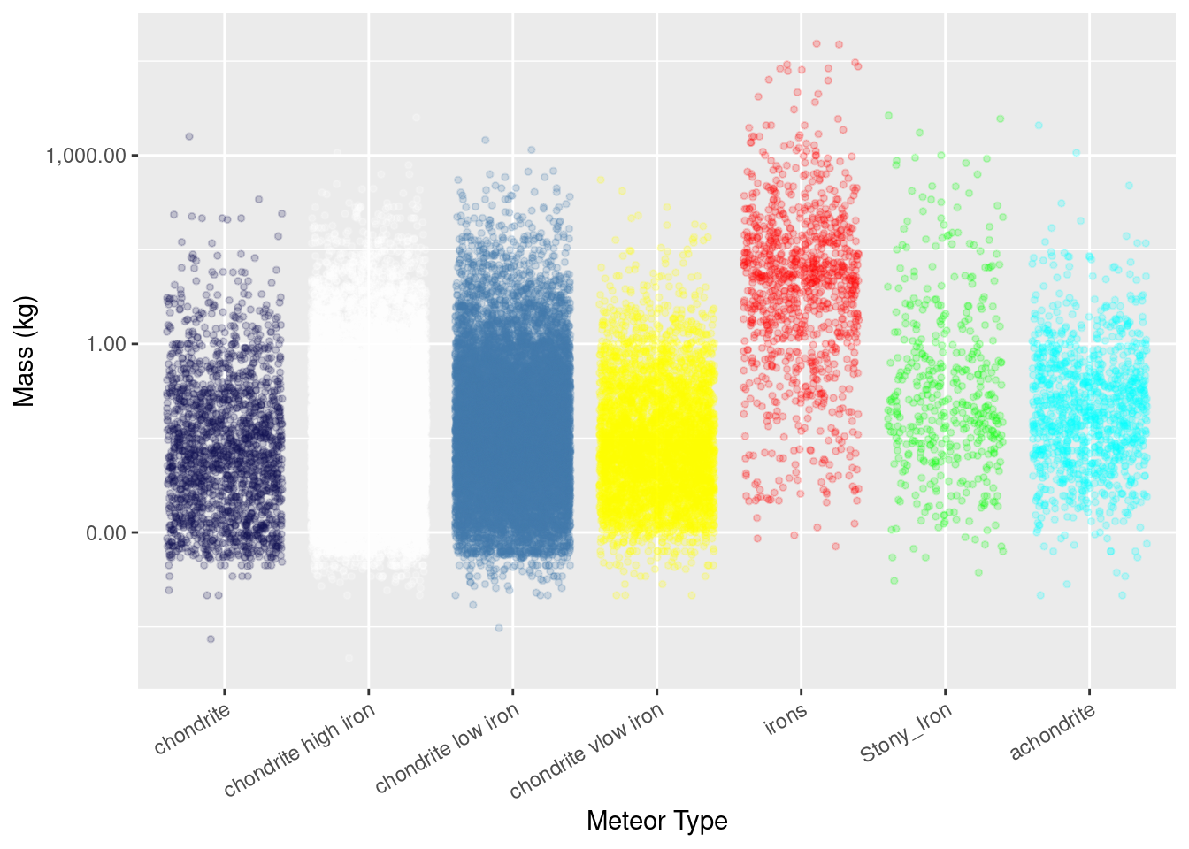
The four classes of chondrite seem to have similar mass distributions, something that can be investigated by an ANOVA test. The result is a p-value of 0.09. Looks like all the chondrites do indeed have similar masses. To have a closer look, a Tukey Test comes up with the following table
| contrast | null.value | estimate | conf.low | conf.high | adj.p.value |
|---|---|---|---|---|---|
| chondrite high iron-chondrite | 0 | -0.49 | -2.32 | 1.34 | 0.90 |
| chondrite low iron-chondrite | 0 | -0.21 | -2.06 | 1.64 | 0.99 |
| chondrite vlow iron-chondrite | 0 | -1.42 | -3.47 | 0.63 | 0.28 |
| chondrite low iron-chondrite high iron | 0 | 0.27 | -0.61 | 1.16 | 0.86 |
| chondrite vlow iron-chondrite high iron | 0 | -0.93 | -2.18 | 0.31 | 0.22 |
| chondrite vlow iron-chondrite low iron | 0 | -1.21 | -2.48 | 0.07 | 0.07 |
From this we see that all types of chondrites have pretty similar masses.
Now let’s see how they spread out across the globe. This is shown in the map below. There are lots of low iron (13434) and high iron (16330) chondrites, so the map will be slow to update and navigate when these are selected. The distribution of most types look similar, with the exception of the irons. My guess is that this is a finding bias, there are terrains like the American mid-West which favour finding a lump of iron but where non-iron meteorites won’t stand out so much. And it just goes to show that there must be umpteen meteorites out there waiting to be picked up.
Finally, Back to those Yamato Meteorites
Did they all come from the same source? Was it one incoming meteoroid that shattered into thousands of peices? If so, they should all have similar compositions. We looked at this, taking the proportional representation of each class in the Yamato field and compared to the overall meteorite population. For good measure, we did this for the Asuka field as well. The results are shown in the table below for the most common classes in the yamato field:
| Meteorite Category | Yamato | all | Asuka | QAR |
|---|---|---|---|---|
| H4 | 0.274 | 0.102 | 0.269 | 0.006 |
| L6 | 0.148 | 0.197 | 0.156 | 0.098 |
| H5 | 0.146 | 0.163 | 0.160 | 0.124 |
| H6 | 0.097 | 0.107 | 0.079 | 0.079 |
| LL6 | 0.038 | 0.044 | 0.030 | 0.027 |
| H4/5 | 0.033 | 0.010 | NA | NA |
| L4 | 0.030 | 0.025 | 0.025 | 0.006 |
| LL | 0.030 | 0.006 | 0.002 | NA |
| E3 | 0.028 | 0.005 | NA | NA |
| L5 | 0.020 | 0.088 | 0.024 | 0.193 |
| H3 | 0.016 | 0.009 | 0.023 | NA |
| L3 | 0.016 | 0.008 | 0.034 | NA |
| CM2 | 0.013 | 0.009 | 0.004 | 0.007 |
| Diogenite | 0.010 | 0.005 | 0.009 | 0.001 |
| LL-melt breccia | 0.007 | 0.001 | NA | NA |
| LL4 | 0.006 | 0.005 | 0.015 | 0.004 |
| Eucrite | 0.005 | 0.003 | 0.005 | NA |
| Eucrite-pmict | 0.005 | 0.004 | 0.002 | NA |
| LL5 | 0.005 | 0.057 | 0.002 | 0.427 |
| LL5/6 | 0.005 | 0.001 | NA | 0.000 |
Yamato and Asuka seem to track each other pretty closely. They do differ significantly from the overall population of meteorites, especially for H4, a high iron chondrite with abundant chondrules. Our guess is that this is simply a collection bias. H4’s are tough to distinguish from regular rocks, but on the Antarctic ice sheet that’s not a big problem.
On the other hand, the Queen Alexandra Range (QAR) meteorites show a significant departure from both the overall meteorite population and also their Antarctic brethren. They have considerably more low iron chondrites (L5 and LL5). Maybe in this case, they are fragments from the same progenitor meteoroid.
To Wrap Up
This is a cursory look at the locations and natures of meteorites. They are fascinating. One thing not discussed is the science that unfolds from meteorite examination. The ability to collect samples from the early Solar System, from diverse sectors of our Solar System, and study them in laboratories here on Earth has revealed rich information about the formation and inner workings of our home. It is an active and fruitful area of research. The staggering number of meteorites being uncovered nowadays mean new insights are inevitable.
Finally. The best place to find meteorites; Antarctica. Barring that, the Sahara. But meteorites are ubiquitous, the best way to find them is to know what you’re looking for by checking out some pictures or by visiting your local museum of natural history.
## R version 4.0.0 (2020-04-24)
## Platform: x86_64-pc-linux-gnu (64-bit)
## Running under: Ubuntu 20.04.1 LTS
##
## Matrix products: default
## BLAS: /usr/lib/x86_64-linux-gnu/blas/libblas.so.3.9.0
## LAPACK: /usr/lib/x86_64-linux-gnu/lapack/liblapack.so.3.9.0
##
## locale:
## [1] LC_CTYPE=en_GB.UTF-8 LC_NUMERIC=C LC_TIME=en_IE.UTF-8
## [4] LC_COLLATE=en_GB.UTF-8 LC_MONETARY=en_IE.UTF-8 LC_MESSAGES=en_GB.UTF-8
## [7] LC_PAPER=en_IE.UTF-8 LC_NAME=C LC_ADDRESS=C
## [10] LC_TELEPHONE=C LC_MEASUREMENT=en_IE.UTF-8 LC_IDENTIFICATION=C
##
## attached base packages:
## [1] stats graphics grDevices utils datasets methods base
##
## other attached packages:
## [1] broom_0.7.1 knitr_1.30 lubridate_1.7.9 rworldmap_1.3-6 sp_1.4-2
## [6] leaflet_2.0.3 forcats_0.5.0 stringr_1.4.0 dplyr_1.0.2 purrr_0.3.4
## [11] readr_1.3.1 tidyr_1.1.2 tibble_3.0.3 ggplot2_3.3.2 tidyverse_1.3.0
##
## loaded via a namespace (and not attached):
## [1] httr_1.4.2 maps_3.3.0 jsonlite_1.7.1
## [4] dotCall64_1.0-0 modelr_0.1.8 assertthat_0.2.1
## [7] memuse_4.1-0 askpass_1.1 highr_0.8
## [10] blob_1.2.1 cellranger_1.1.0 yaml_2.2.1
## [13] remotes_2.2.0 pillar_1.4.6 backports_1.1.10
## [16] lattice_0.20-41 glue_1.4.2 digest_0.6.25
## [19] RColorBrewer_1.1-2 rvest_0.3.6 leaflet.providers_1.9.0
## [22] colorspace_1.4-1 rprofile_0.1.4.9002 htmltools_0.5.0
## [25] clisymbols_1.2.0 pkgconfig_2.0.3 haven_2.3.1
## [28] bookdown_0.20 scales_1.1.1 openssl_1.4.3
## [31] farver_2.0.3 generics_0.0.2 ellipsis_0.3.1
## [34] withr_2.3.0 credentials_1.3.0 cli_2.1.0
## [37] magrittr_1.5 crayon_1.3.4 readxl_1.3.1
## [40] memoise_1.1.0 maptools_1.0-2 evaluate_0.14
## [43] fs_1.5.0 fansi_0.4.1 xml2_1.3.2
## [46] foreign_0.8-80 blogdown_0.20 tools_4.0.0
## [49] hms_0.5.3 lifecycle_0.2.0 gert_0.3
## [52] munsell_0.5.0 reprex_0.3.0 compiler_4.0.0
## [55] rlang_0.4.8 grid_4.0.0 rstudioapi_0.11
## [58] sys_3.4 htmlwidgets_1.5.2 spam_2.5-1
## [61] crosstalk_1.1.0.1 prompt_1.0.0 labeling_0.3
## [64] rmarkdown_2.4 gtable_0.3.0 DBI_1.1.0
## [67] R6_2.4.1 stringi_1.5.3 parallel_4.0.0
## [70] Rcpp_1.0.5 fields_11.5 vctrs_0.3.4
## [73] dbplyr_1.4.4 tidyselect_1.1.0 xfun_0.18