Where to find your Genes

We’ve been working with the genetics of schizophrenia, looking at how the expression of genes that play a role in the condition vary across brain regions and neurodevelopment stages. Now, call me old-fashioned, but I like to know how things are laid out, so in this case where these genes are situated. Time for a plot.

The genes in question come from a GWAS study of the PGC. The images are build based on the ggbio and karyoploteR packages from bioconductor.

First, let’s load up the required packages:

knitr::opts_chunk$set(echo = TRUE, message = FALSE, warning = FALSE)

if (!require("pacman")) install.packages("pacman")

## Loading required package: pacman

pacman::p_load(annotables, tidyverse, ggbio,
               httr, readxl, ABAData, 
               GenomicRanges, karyoploteR)

Next, we get a list of the genes from the PGC. These are taken from one of the supplementary tables from the 2018 paper mentioned above. We only care about the ones that also feature in the Allen Brain Atlas, so we filter for those.

url <- "https://www.ncbi.nlm.nih.gov/pmc/articles/PMC5918692/bin/NIHMS958804-supplement-Supplementary_Table.xlsx"
GET(url, write_disk(temp_file <- tempfile(fileext = ".xlsx"))) # downloads the .xlsx file

## Response [https://www.ncbi.nlm.nih.gov/pmc/articles/PMC5918692/bin/NIHMS958804-supplement-Supplementary_Table.xlsx]
##   Date: 2020-10-25 03:00
##   Status: 200
##   Content-Type: application/vnd.openxmlformats-officedocument.spreadsheetml.sheet
##   Size: 1.27 MB
## <ON DISK>  /tmp/Rtmpw0u1Yv/file23c4d3437ffbc.xlsx

df <- read_excel(temp_file, sheet = 4, skip = 3) # reads into a dataframe. First six rows of the excel file are just header
unlink(temp_file)     # deletes the temporary file


##################################################################
# makes sz_genes, a dataframe with a single column of the CLOZUK genes
#######################################################################

sz_genes <- df$`Gene(s) tagged` %>% 
  str_split(",") %>% 
  unlist() %>% 
  as.data.frame() %>% 
  distinct()
names(sz_genes) <- "genes"


data("dataset_5_stages")

genes <- sz_genes %>% 
  semi_join(dataset_5_stages, by = c("genes" = "hgnc_symbol")) %>% 
  pull(genes)

From our gene list we build a data frame of gene information using Human build 38 (grch38 from the annotables package). And then turn his into an appropriate GRanges object (thank you GenomicRanges).

gene_table <- grch38 %>% 
  dplyr::filter(symbol %in% genes) %>% 
  dplyr::filter(chr %in% c(1:22, "X", "Y")) %>% 
  dplyr::mutate(strand = ifelse(strand == 1, "+", "-"))

gene_ranges <- makeGRangesFromDataFrame(gene_table, keep.extra.columns = T)
seqlevelsStyle(gene_ranges) <- "UCSC"

Now for the plot. The plotKaryotype() function does a lqyout of 24 chromosomes with their cytobands, the kpPlotMarkers() adds in the gene labels. The label colours depend on strand; red for + and green for -. I wasn’t too successful avoiding label overlaps, sorry about that.

kp <- plotKaryotype(genome="hg38")
kpPlotMarkers(kp, 
              data=gene_ranges, 
              labels=gene_ranges$symbol, 
              label.color = ifelse(gene_table$strand == "+", "darkred", "olivedrab4"),
              text.orientation = "horizontal",
              label.dist = 0.0001,
              r1=0.5, cex=0.6, adjust.label.position = T)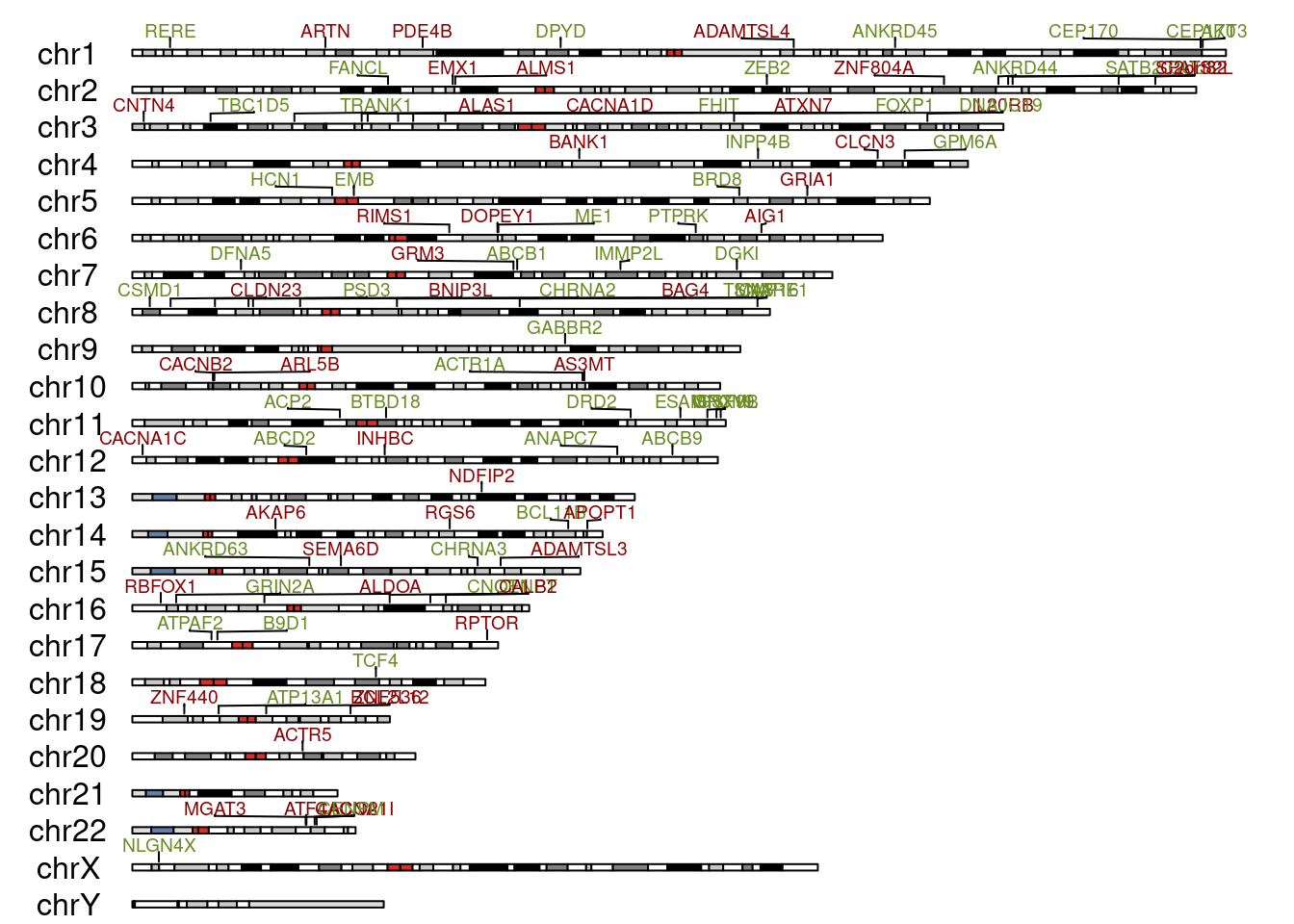

Our genes are pretty spread out with no particular pattern of course. But I just feel I know them a little better now.